At a glance
AI Revolution walks through a single Nature paper from Google Quantum AI and Google DeepMind, and the fifteen minutes are unusually dense with real physics. The paper is Reinforcement learning control of quantum error correction, first posted as arXiv:2511.08493 and written up by Google as Towards a quantum computer that learns from its errors. The result: on a Willow superconducting processor, a reinforcement learning agent watches the error correction system's own detection events, works out which of thousands of control knobs have drifted, and retunes them while the computation keeps running.
The numbers the video reports are all in the paper. On a processor already calibrated by the full automated stack plus human experts, the agent found another 20% suppression of the logical error rate. Under artificially injected drift it delivered a 24% reduction and a 2.4 fold improvement in stability, rising to 31% and 3.5 fold once it was allowed to steer the decoder's parameters too. The record numbers from the same work: an average logical error per cycle of 7.72(9) × 10⁻⁴ for the distance 7 surface code and 8.19(14) × 10⁻³ for the distance 5 color code. Simulations of a distance 15 code with roughly 40,000 control parameters showed the number of training epochs needed is independent of system size.
The framing the narrator lands on at the end is the interesting part, and it is a fair reading of the paper: the road to fault tolerance was always assumed to be a hardware story about better fabrication and more qubits. This says a meaningful chunk of it is a control story, and control is exactly the kind of problem machine learning is good at. What follows is the whole video rebuilt in order, with every number, every named system, and every source linked.
Chapters
- 00:02 The claim, stated precisely
- 00:38 The real problem is not fragility, it is that the machine is analog
- 01:38 The orchestra that keeps going out of tune
- 01:53 How the field handles it today: kill the computation
- 02:20 Why that breaks for the algorithms anyone actually wants
- 02:40 The machinery you need first: quantum error correction
- 03:24 Detection events are vague, and that is what decoders are for
- 03:59 The gap: the decoder tells you what to fix, never why
- 04:07 Decoherence you cannot fix, calibration you can
- 04:37 A short break, and a script slip
- 05:14 The old way: decades of physics and a calibration graph
- 05:53 Hand built models hit ceilings, and that is a pattern
- 06:38 The idea: give the detection data a second job
- 07:23 The hurdle: you cannot optimize the number you actually care about
- 07:49 The proxy: average detection event rate
- 08:08 Sparsity is the real unlock
- 08:34 Under the hood: policy gradients pointed at superconducting hardware
- 09:01 Result one: another 20% on top of expert calibration
- 09:38 Record numbers
- 10:06 Result two: they broke it on purpose
- 11:04 Against the drift the chip does on its own
- 11:14 The stress test: scramble it and watch it come back
- 11:37 The same trick, already reused
- 11:47 Does it scale
- 12:26 The one genuine limitation
- 13:07 Where this goes next
- 13:44 The reframe: fault tolerance is partly a control story
The claim, stated precisely (00:02)
The video opens with a careful piece of expectation management, which is not what you normally get from a channel with "Massive Breakthrough" in the title. Google may have just solved one of quantum computing's most frustrating problems by giving the machine the ability to learn from its own mistakes while it is still running. But to be clear, the narrator says, this does not mean the Willow chip can physically repair a broken wire or rebuild a damaged qubit.
What it means is arguably more important. The system can now notice when its controls are drifting out of alignment, figure out which settings are causing the trouble, and retune itself without shutting the computation down.
That is a bigger deal than it sounds, and to see why you have to look at one of quantum computing's biggest problems, which, the narrator promises, is probably not the one you have in mind.
The real problem is not fragility, it is that the machine is analog (00:38)
Everyone knows qubits are fragile. That is the headline everyone repeats, and it is the wrong place to put the emphasis.
The deeper issue is that a quantum computer is an analog machine. Your laptop is digital. Everything is a clean one or a zero, and a little bit of electrical noise gets rounded away like it never happened. That rounding is a mercy, and a quantum processor does not get it.
The qubits are controlled by physical microwave signals. Every one of those signals has a frequency, an amplitude, and a phase, and all of those numbers have to be dialed in with absurd precision. Not close enough. Exact.
And here is the problem: those numbers do not stay put. The hardware drifts. Temperature in the control electronics shifts slightly. Material defects near the chip shuffle around. The qubits themselves change their behavior over time. So a set of control parameters that was perfect an hour ago is quietly wrong now, and every gate you run with those stale values is injecting fresh errors into your computation.
This is the part that gets lost in the popular framing. It is not that the qubit is delicate in some abstract way. It is that the instrument goes out of tune while you are playing it, and nothing rounds the mistuning away.
The orchestra that keeps going out of tune (01:38)
The analogy the narrator reaches for is an orchestra where the violins slide out of tune every couple of measures. The music does not stop because the players are bad. It stops because you have to keep retuning.
That, right now, is the actual operational reality of running a quantum computer. Not a metaphor for it. The reality.
How the field handles it today: kill the computation (01:53)
The way the field has dealt with this up to now is, in the narrator's word, brutal. You kill the computation. You shut the whole thing down. You run your calibration routines. You tune everything back up. Then you start over.
Which is completely fine when your experiment lasts a few seconds.
Why that breaks for the algorithms anyone actually wants (02:20)
It is a catastrophe when your experiment does not last a few seconds. The algorithms people actually want quantum computers for, simulating chemical reactions, breaking RSA encryption with Shor's algorithm, that tier of problem, are not seconds long jobs. Estimates put them at days, sometimes months of continuous run time. Google's own 2025 resource estimate for factoring a 2048 bit RSA integer puts the runtime for that specific job on the order of a week on a million noisy qubits, and chemistry problems run longer.
You cannot stop a computation that runs for a month every time your hardware sneezes.
So calibration and computation being two separate, mutually exclusive modes is not an inconvenience. It is a hard wall standing between us and anything useful. The question the whole paper answers: how do you tune the instruments while the music is still playing?
The machinery you need first: quantum error correction (02:40)
Before the answer there is a piece of machinery you have to understand, because the whole trick depends on it: quantum error correction.
The core problem with fixing errors on a quantum computer is that looking at a qubit destroys it. Measuring it collapses the superposition. So you cannot just peek and check whether everything is okay. The act of checking is the damage.
The workaround is redundancy. You take a whole bunch of physical qubits and weave them together into one much more robust logical qubit, using a code like the surface code or the color code. Then you run specialized parity checks that never touch the actual information. Those checks give you binary output. Error, or no error.
That is the whole magic of the scheme, and the narrator states it well: it is how you take messy analog noise and turn it into something digital you can actually reason about.
Detection events are vague, and that is what decoders are for (03:24)
The catch is that these signals are vague. A detection event tells you an error happened somewhere inside a bounded region of space and time in your circuit. It does not tell you where.
You hear a sour note. You have no idea which musician played it.
That is what decoders are for. Google has two of them in this story:
- AlphaQubit, a neural network decoder trained on real hardware data, published in Nature in November 2024, and its successor AlphaQubit 2, which decodes both surface and color codes in real time.
- Tesseract, an algorithmic most likely error decoder that runs an A* search over an exponentially large graph of error hypotheses to find the most probable pattern.
Feed either one the detection events, it infers what probably went wrong, and it hands you back the correction. If errors stay rare enough, the logical information survives.
The gap: the decoder tells you what to fix, never why (03:59)
Now notice what is missing. The decoder tells you what to fix. It never tells you why it happened.
The narrator flags this as the whole story, and he is right. That gap is exactly the hole the paper fills.
Decoherence you cannot fix, calibration you can (04:07)
Some of the errors are unavoidable. Decoherence, the quantum system leaking into its environment, is fundamental physics. It is the same process responsible for why the world looks classical to us at all. You cannot engineer that away.
But a huge chunk of the remaining errors are just bad calibration. Control parameters that have drifted. Signals that are slightly off. Those are entirely within our power to fix, and here is the sentence the whole paper hangs on: every single one of them is already showing up in the detection data as a symptom that nobody was reading.
The data was sitting there the entire time. It was being consumed for exactly one purpose and then thrown away.
A short break, and a script slip (04:37)
The video takes a sponsor break here, and it is worth reporting honestly because it is part of the video. The channel is giving away a guide to seven AI agents that businesses are reportedly paying $3,000 to $10,000 for, chosen by an audience poll the previous day. The pitch covers what the agents cost, who needs them, how to spot the right clients, the ROI, setup fees, retainers, and what a realistic $10,000 per month client list could look like with zero coding required. The link is go.aiskool.io/7agents, which is also in the video description.
Then comes the funniest thirty seconds of the video, and it is unintentional. The narrator says: "All right, now back to Anthropic. All right, now back to the video." Two returns from the break, back to back, with the wrong one first. Whatever templated ad read this channel reuses across videos, the tail of an Anthropic segment survived the edit and made it into the final cut. If you want a small window into how a daily AI news channel is actually produced, that is it.
The old way: decades of physics and a calibration graph (05:14)
Back to the science. The traditional response to calibration was physics, decades of it.
You build an accurate model of the system. You isolate parameters so they do not interfere with each other. You design dedicated experiments that target a few at a time. Want to calibrate the frequency of a microwave pulse? Spectroscopy. Want the amplitude? Rabi oscillations.
Google eventually formalized the whole thing into an automated framework. In the 2018 paper Physical qubit calibration on a directed acyclic graph, Julian Kelly, Peter O'Malley, Matthew Neeley, Hartmut Neven and John Martinis reduced calibration to a graph traversal problem: each calibration routine is a node in a directed acyclic graph, and the edges encode the bootstrapping order in which everything has to be tuned. Decades of quantum control research, distilled into a walkable graph.
It works. It has gotten Google to the scale of a few hundred qubits. But hand built models hit ceilings.
Hand built models hit ceilings, and that is a pattern (05:53)
The narrator makes the point that this is not a quantum thing. It is a pattern, and he lists three cases:
- Early computer vision stalled out trying to describe the world with rigid geometric rules.
- Robotics still fights with kinematic equations that fall apart the moment real friction and contact dynamics enter the picture.
- Protein folding was considered basically intractable for physics based modeling until AlphaFold showed up and just learned it from data instead.
Every one of those broke open the same way. And quantum control was sitting right at that ceiling.
The specific reason is worth keeping. As chips get better, the errors that remain are the weird ones. Exotic, low probability channels that come from the simplifying assumptions baked into your model, or from device physics nobody has characterized yet. Your model cannot fix what it does not know exists.
The idea: give the detection data a second job (06:38)
Which brings us to the actual idea, and the narrator's assessment of it is the best line in the video: it is elegant enough that it is slightly infuriating nobody did it sooner.
The quantum error correction process is already generating a continuous stream of error detection events, constantly, for free, as a byproduct of running at all. That data is already being used for decoding. So Google gave it a second job.
Same data, two roles. It still goes to the decoder to correct the logical state. But it also gets fed to a reinforcement learning agent as a training signal. The agent watches which detectors are lighting up, deliberately applies tiny perturbations across all the control parameters at once, and learns to correlate specific nudges with specific changes in performance.
Cause and effect teased apart from noise, continuously, while the computation runs.
The hurdle: you cannot optimize the number you actually care about (07:23)
There is a real technical hurdle buried in that picture, and the video does not skip it.
The number you actually care about is the logical error rate. You cannot optimize against it directly, for three separate reasons:
- It is suppressed exponentially with code size, which means measuring it accurately takes an exponentially huge number of cycles.
- It is a single scalar, and you are trying to steer thousands of parameters with it. One number cannot tell thousands of knobs apart.
- During a real computation you do not even know the logical state, so you cannot compute it.
Any one of those would be bad. All three together kill the direct approach outright.
The proxy: average detection event rate (07:49)
So they optimize a proxy instead: the average rate of error detection events across every detector in the circuit.
That is cheap to measure, it is local, and it tracks the thing you care about closely enough that the math works out. The paper's version of "closely enough" is a clean proportionality between the gradients, tied to the code distance. In the preprint's notation, the gradient of the log logical error rate equals (d + 1) / 2 times the gradient of the log detection rate, where d is the code distance. They did not just assert it. They confirmed it experimentally.
The cost advantage is the real point. Measuring the proxy takes a number of cycles that scales with the inverse of the detection rate and is independent of code distance, while measuring the logical error rate itself gets exponentially more expensive as the code gets bigger.
Sparsity is the real unlock (08:08)
The proxy makes the objective measurable. Sparsity is what makes the optimization tractable.
Each detector only cares about the handful of gates inside its own little region of the circuit. Errors are local, and detection events inherit that locality. So instead of one impossible thousand dimensional optimization problem, you get a sprawling graph of thousands of tiny, mostly independent ones.
On the distance 5 surface code they ran, the structure comes out like this: each detector connects to about 302 parameters, and each parameter touches roughly 18 detectors. That is a sparse factor graph, not a dense mess, and the narrator is explicit that this structure is why the thing scales at all.
Under the hood: policy gradients pointed at superconducting hardware (08:34)
Mechanically it is a policy gradient setup, and the video runs through the ingredients without hedging.
The agent samples a batch of candidate control policies from a probability distribution, a factorized multivariate Gaussian with an evolving mean and covariance. It ranks them by which produced fewer detection events. Then it nudges the distribution toward the winners. On top of that:
- Proximal policy optimization for stability, so no single update yanks the policy somewhere destructive.
- Entropy regularization so the agent never stops exploring and never collapses onto a stale local optimum.
- A replay buffer for sample efficiency, because shots on a quantum processor are expensive.
The narrator's summary is exactly right and worth keeping: standard modern reinforcement learning, pointed at superconducting hardware. None of the machine learning is exotic. The novelty is entirely in what the reward signal is and where it comes from.
Result one: another 20% on top of expert calibration (09:01)
They ran this on Willow, and they ran it in two very different ways.
The first experiment is the hardest possible test of "is there anything left on the table." Take a processor that has already been calibrated within an inch of its life: the full traditional automated stack, plus extensive human expert tuning, actual scientists applying physical intuition to the edge cases you cannot automate. Then turn the agent loose on top of that.
It found another 20% suppression of the logical error rate, consistently, across multiple independent runs, on both the surface code and the color code.
The narrator lets that land: 20% of performance that decades of quantum control theory and human expertise had simply left on the table. Not 20% over a naive baseline. Twenty percent over the best the field knew how to do by hand.
Record numbers (09:38)
That pushed them to record numbers, and these are the ones to write down:
- The distance 7 surface code hit an average logical error rate of 7.72 × 10⁻⁴ per cycle, decoded with AlphaQubit 2. That is fewer than one logical error per thousand error correction cycles.
- The distance 5 color code came in at 8.19 × 10⁻³, decoded with Tesseract. Roughly one per hundred.
The paper's abstract gives them with uncertainties as 7.72(9) × 10⁻⁴ and 8.19(14) × 10⁻³. The narrator's claim about them: best anyone has demonstrated on any qubit platform, full stop.
Result two: they broke it on purpose (10:06)
The second experiment is the one that actually tests the premise, because a one time 20% polish does not prove anything about drift. So they injected artificial drift straight into the control parameters.
The shapes of drift they injected:
- Step changes, a sudden jump in a parameter.
- Slow sine waves, gradual oscillating drift.
- Stroboscopic pulses.
And the targets they injected into: CZ coupling strengths, and XY pulse amplitudes and frequencies, at different spots on the qubit grid.
A fixed control policy degrades exactly the way you would expect, error rates climbing as the parameters go stale. The agent tracks the drift and holds the detection rate below where it started.
When they slammed a step function change into a pulse amplitude, recovery took about 130 learning epochs. That is the concrete number for how fast this thing reacts, and it is the one you need to hold onto for the limitation section later.
In logical terms, steering the control parameters produced a 24% reduction in error rate and a 2.4 fold improvement in stability. Then they took it further and let the agent steer the decoder's parameters too, and those jumped to 31% and a 3.5 fold improvement.
Against the drift the chip does on its own (11:04)
Injected drift is a controlled test. The chip also drifts naturally, on its own, from all the causes listed at the top: electronics temperature, defects shuffling, qubits changing character.
Fourier analysis of the experimental runs showed that the steering behaves like a filter, knocking a few decibels off the low frequency fluctuations in the logical error rate. The video says about four decibels. The November preprint says about six. Either way the qualitative result is the same and it is the useful one: the agent is not just cleaning up the artificial drift you injected, it is suppressing the real slow wander of the machine.
The stress test: scramble it and watch it come back (11:14)
Then they ran a test the narrator calls borderline showing off, and it is the most interesting result in the paper for anyone thinking about where this goes.
They randomized the control policy, deliberately scrambling it badly enough that the logical observable was completely destroyed. Not degraded. Destroyed. And the agent found its way back to high performance from scratch. In the preprint's own words, it "successfully recovers the performance after we artificially randomize the control policy to fully scramble the logical observable, mimicking a coarse calibration scenario."
Which hints at something much bigger than fine tuning. It suggests reinforcement learning could eventually replace whole chunks of the calibration stack rather than just polishing its output. The agent did not need a good starting point. It needed a signal and some knobs.
The same trick, already reused (11:37)
The technique is not sitting in one paper. It already got used in Google's magic state cultivation work, the scheme for producing the non Clifford resource states that a fault tolerant machine burns through by the millions. There it delivered an order of magnitude improvement in cultivation error and post selection rate.
That is a good sign for generality. The same optimizer, pointed at a different part of the fault tolerance stack, produced a 10× result rather than a 20% one.
Does it scale (11:47)
Then comes the question everyone asks about anything involving machine learning and quantum hardware. Does it scale?
They simulated a distance 15 surface code, roughly 40,000 control parameters at about 30 per gate. And the finding is the good one.
The number of training epochs the agent needs is independent of system size. Not "scales gently." Independent.
The reason is the sparsity from earlier. Because detection events are local, adding more qubits adds more subproblems, but does not make any individual subproblem harder. The convergence follows a clean exponential law, and the rate depends on how many parameters each gate has, not on how big the machine is.
This is the single most load bearing claim in the paper for anyone thinking about the road to a million qubits, and it is the one the abstract chose to highlight: "an optimization speed that is independent of system size."
| calibrate, then compute | learn while computing | |
|---|---|---|
| What happens when the hardware drifts | Terminate the computation, run calibration routines, tune back up, start over. | Nothing stops. The agent tracks the drift and retunes in place. |
| Where the information comes from | Dedicated experiments designed by physicists: spectroscopy for frequency, Rabi oscillations for amplitude. | The error correction detection events the machine is already producing for free. |
| What is being optimized | Individual parameters, isolated so they do not interfere, in a fixed order set by a directed acyclic graph. | All parameters at once, against the average detection event rate as a proxy for logical error rate. |
| Human involvement | Decades of quantum control theory, plus expert scientists on the edge cases. | The agent found another 20% on top of exactly that. |
| Errors it can address | Only the ones the physical model knows about. | Anything that moves the detection rate, including channels nobody has characterized. |
| Cost to a month long algorithm | Fatal. Every recalibration kills the run. | Zero downtime, at the cost of exploration noise. |
| Scaling behavior | Has carried Google to a few hundred qubits. | Training epochs independent of system size, verified in simulation to distance 15 and 40,000 parameters. |
The one genuine limitation (12:26)
There is one genuine limitation, and the video credits the authors for being upfront about it.
Learning requires exploration, and exploration means sometimes running policies that are worse than your current best.
In these experiments that is harmless, because the quantum state gets re-prepared every shot. Run a bad policy, throw away the shot, no lasting damage. But during a single long algorithm, that exploration noise is real damage to the actual computation you are trying to protect.
So there is a trade off, and the simulations put a number on it. They found a critical drift frequency around 1 over 150 epochs. Below that, the trade off comes out in your favor and real time steering beats a fixed policy. Above it, the agent simply cannot keep up, and the exploration cost exceeds the benefit.
The narrator names one thing that falls on the wrong side of that line: cosmic ray strikes and high energy particle impacts, which hit a large fraction of the chip at once and are far too fast for a 150 epoch response. Those have to be handled in hardware, and Google has separate work on exactly that.
Where this goes next (13:07)
Right now the agent uses a simple Gaussian policy. Not because anything fancier failed, but purely because the data rate between the chip and the classical controller is too slow to train anything fancier. The bottleneck is plumbing.
Speed up that loop and the ceiling moves:
- Put a deep neural network in there instead of a Gaussian.
- Condition it on what the detectors are actually reporting rather than treating them as a scalar reward.
- Have it learn a model of the system alongside the policy, and start surfacing correlations nobody knew were there.
The end game the authors float is the one the stress test already gestured at: a processor calibrated for error correction entirely from scratch by the agent. No physics models. No human experts. No calibration graph.
The reframe: fault tolerance is partly a control story (13:44)
The framing the narrator keeps coming back to, and the reason this is worth fifteen minutes of your time, is that none of this requires anything special about superconducting circuits.
All it needs is error detection signals and knobs you can turn. Trapped ions, neutral atoms, whatever comes next. The same idea drops straight in.
The path to fault tolerance was always assumed to be a hardware story. Better fabrication, cleaner materials, more qubits. This says a meaningful chunk of it is a control story, and control is exactly the kind of thing machine learning eats for breakfast.
The video signs off by noting the paper is open access in Nature and dropping the link in the description.
The lineage this sits on
The paper does not arrive out of nowhere. Almost every component in it is a previously published Google result, and the contribution is the wiring.
- 2012Austin Fowler and colleagues publish Surface codes: towards practical large scale quantum computation, the roadmap the whole program has followed since.
- 2018Julian Kelly and colleagues formalize calibration as a graph traversal in Physical qubit calibration on a directed acyclic graph. This is the "old way" the RL agent is measured against, and it is still what gets the processor into the right neighborhood.
- 2024September: Magic state cultivation, later one of the first places the same RL technique gets reused, where it delivers an order of magnitude improvement.
- 2024November: AlphaQubit, the neural network decoder, appears in Nature.
- 2024December: Willow is announced alongside Quantum error correction below the surface code threshold, the first demonstration that adding qubits makes the logical qubit better rather than worse. The same month brings Scaling and logic in the color code on a superconducting quantum processor.
- 2025March: the Tesseract search based most likely error decoder.
- 2025November: the preprint at the center of this video, Reinforcement Learning Control of Quantum Error Correction, goes up on arXiv with an author list running to several hundred names.
- 2025December: AlphaQubit 2, a scalable real time neural decoder for both surface and color codes, the decoder credited with the record surface code number.
- 2026July: Nature publishes Reinforcement learning control of quantum error correction. Google posts its own explainer, and the trade and science press picks it up.
Best quotes
"This does not mean Google's Willow chip can physically repair a broken wire or rebuild a damaged qubit. What it means is arguably more important." (00:12)
"Everyone knows qubits are fragile. That's the headline everyone repeats. The deeper issue is that a quantum computer is an analog machine." (00:38)
"All of those numbers have to be dialed in with absurd precision. Not close enough, exact." (01:08)
"Think about an orchestra where the violins slide out of tune every couple of measures. The music doesn't stop because the players are bad. It stops because you have to keep retuning." (01:38)
"You cannot stop a computation that runs for a month every time your hardware sneezes." (02:25)
"The core problem with fixing errors on a quantum computer is that looking at a qubit destroys it. The act of checking is the damage." (02:49)
"You hear a sour note, you have no idea which musician played it." (03:35)
"The decoder tells you what to fix. It never tells you why it happened. And that gap is the whole story here." (04:01)
"Every single one of them is showing up in the detection data as a symptom that nobody was reading." (04:33)
"All right, now back to Anthropic. All right, now back to the video." (05:11)
"Your model can't fix what it doesn't know exists." (06:34)
"And it's elegant enough that it's slightly infuriating nobody did it sooner." (06:40)
"Same data, two roles." (06:54)
"Cause and effect teased apart from noise continuously while the computation runs." (07:17)
"20% of performance that decades of quantum control theory and human expertise had simply left on the table." (09:31)
"Second experiment. They broke it on purpose." (10:06)
"They also ran a stress test that's borderline showing off." (11:14)
"The number of training epochs the agent needs is independent of system size, not scales gently, independent." (12:02)
"The end game they float is a processor calibrated for error correction entirely from scratch by the agent. No physics models, no human experts, no calibration graph." (13:32)
"The path to fault tolerance was always assumed to be a hardware story. Better fabrication, cleaner materials, more qubits. This says a meaningful chunk of it is a control story and control is exactly the kind of thing machine learning eats for breakfast." (14:01)
Where it stands
An honest accounting, saved for the end because the video's own framing is worth taking on its own terms first.
The science is real and it is peer reviewed. This is not a press release. It is a Nature paper with an author list that runs to several hundred names, essentially the whole of Google Quantum AI plus collaborators at Google DeepMind, led by Volodymyr Sivak and Paul Klimov. Every number the video quotes is in the paper or its abstract. The Quantum Insider, phys.org and Ars Technica all covered it independently within the same window.
Where the video is slightly loose. Two small things. It says the natural drift filtering knocks about four decibels off low frequency fluctuations; the November preprint says about six. And the record numbers moved between the preprint and the published version: the arXiv v1 reported a logical error rate of 1.9 × 10⁻³ for the surface code and 0.9 × 10⁻² for the color code using a most likely error hypergraph decoder, while the Nature abstract reports the better 7.72 × 10⁻⁴ and 8.19 × 10⁻³ figures. The video's attribution of those to AlphaQubit 2 and Tesseract respectively matches Google's own blog post and the AlphaQubit 2 paper, but it is worth knowing the paper grew between preprint and publication.
What "breakthrough" does and does not mean here. No new chip. No new qubit count. No claim of quantum advantage on a useful problem. What actually changed is that a mode switch which everyone assumed was mandatory turned out not to be. That is a genuine unlock for long algorithms, and it is also an incremental engineering result, and both of those are true at once. The 20% figure is the honest headline: it is a large number in a field where single digit improvements are worth publishing, and it is a percentage improvement on an error rate, not a change in kind.
The limitation is the real one. Exploration noise during a single long algorithm is not a footnote, it is the thing standing between this demonstration and the use case it is motivated by. The paper says so plainly and gives the number: below a drift frequency of roughly 1 over 150 epochs the trade comes out in your favor, above it the agent cannot keep up. Cosmic ray events sit on the wrong side of that line. So the honest statement of what was demonstrated is: continuous recalibration works, and the regime where it beats a fixed policy has a measured boundary.
What to actually watch next. The scaling claim, that training epochs are independent of system size, is verified in simulation and not yet on hardware at distance 15. The from scratch calibration end game is a supplementary material result on a scrambled policy, not a production capability. And the near term bottleneck the authors name is unglamorous: the classical data rate between the chip and its controller. If that gets faster, the Gaussian policy becomes a neural network and this gets considerably more interesting.
Resources
The paper and Google's own writeups
- Reinforcement learning control of quantum error correction, Nature, 2026. DOI 10.1038/s41586-026-10759-2. Open access.
- arXiv:2511.08493, the November 2025 preprint, with the full PDF.
- Towards a quantum computer that learns from its errors, the Google Research blog post by Volodymyr Sivak and Paul Klimov.
- Google Quantum AI and Google DeepMind, the two groups behind the work.
Press coverage of this result
- Google study shows quantum computer can learn from its own errors while it computes, The Quantum Insider, by Matt Swayne.
- Faster, more stable quantum computing, the writeup on Phys.org.
- Quantum error correction can constantly recalibrate a processor, Ars Technica.
The hardware and the codes
- Meet Willow, our state of the art quantum chip, the December 2024 announcement.
- Quantum error correction below the surface code threshold, Nature, the Willow result that made scaling worthwhile.
- Surface codes: towards practical large scale quantum computation, Fowler et al., the foundational surface code paper.
- Scaling and logic in the color code on a superconducting quantum processor, the color code work.
- Magic state cultivation, where the same RL technique produced an order of magnitude gain.
- Resolving catastrophic error bursts from cosmic rays in large arrays of superconducting qubits, Nature Physics, on the failure mode that has to be handled in hardware.
The decoders
- AlphaQubit: learning high accuracy error decoding for quantum processors, Nature, November 2024.
- A scalable and real-time neural decoder for topological quantum codes, the AlphaQubit 2 paper.
- Tesseract: a search based decoder for quantum error correction, and its follow up on accelerating the Tesseract decoder.
The old calibration stack
- Physical qubit calibration on a directed acyclic graph, Kelly, O'Malley, Neeley, Neven and Martinis, 2018.
The machine learning ingredients
- Proximal policy optimization algorithms, Schulman et al.
- Asynchronous methods for deep reinforcement learning, Mnih et al., the entropy regularization reference.
- Playing Atari with deep reinforcement learning, Mnih et al., where the replay buffer comes from.
- Policy gradient methods, background.
- AlphaFold and its Nature paper, the analogy the video leans on for "hand built models hit ceilings."
Background concepts
- Quantum error correction, logical qubit, quantum superposition, decoherence, the quantum threshold theorem.
- Superconducting quantum computing, trapped ion quantum computers, neutral atom quantum computers.
- Rabi cycle, quantum logic gates, directed acyclic graphs, Fourier analysis.
- Shor's algorithm, RSA, and Craig Gidney's 2025 resource estimate for factoring 2048 bit RSA integers.
From the video description
- The channel's free seven agent guide, the sponsored segment at 04:37.
- AI Revolution on YouTube.