At a glance
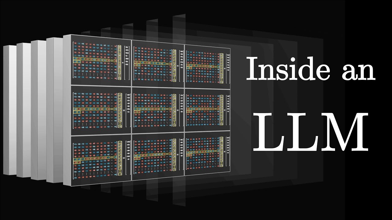
Chapter 5 of the 3Blue1Brown deep learning series followed a stream of data through a transformer and treated attention as a box. Chapter 6 opens the box. Grant Sanderson takes the attention mechanism apart one matrix at a time: the query and key matrices and the geometric meaning of their dot product, the softmax that turns raw scores into an attention pattern, the mask that stops a token from reading the future, the value matrix that actually moves meaning between positions, and finally multi headed attention, which is just many of these running in parallel with different learned specialties.
What makes the episode land is the running parameter tally. Every matrix he introduces gets counted against the real dimensions of GPT-3, so the abstractions never float free of the machine. The motivating example is one sentence, "a fluffy blue creature roamed the verdant forest," and the question of how the adjectives get baked into the noun they modify. Attention is the answer to exactly that question.
This page rebuilds the derivation in the video's order and keeps the numbers.
The deep explanation
The problem attention solves
After the embedding step, each token in the sequence has a vector attached to it, and at that point the vector encodes only the token itself plus its position. It knows nothing about context. That is a problem, because the meaning of a word in a sentence is mostly context. "Model" in "a machine learning model" and "model" in "a fashion model" start life as the same vector.
Sanderson's example is a noun with adjectives in front of it. The vector for "creature" should end up meaning something closer to a fluffy blue creature than to a generic creature. The information is right there in the sequence, sitting on other tokens. Attention is the mechanism that moves it.
The framing he uses: each vector gets to ask a question of every other vector, and the ones with a relevant answer get to update it. Concretely, the network computes for every position a query and a key, compares them, and uses the comparison to decide how much each position should influence each other position.
Queries and keys
The query is produced by multiplying the token's embedding by a learned query matrix. Think of that as encoding a question. For a noun, one plausible learned question is "are there any adjectives sitting in front of me?"
The key is produced by a different learned matrix. Think of it as advertising what a token has to offer. If the query for "creature" is asking for adjectives, then the keys for "fluffy" and "blue" should be the vectors that answer it.
The comparison is the dot product between a query and a key: large and positive when they point the same way, near zero when unrelated. Compute it for every query against every key and you get a grid of scores, one per pair of positions. In the fluffy blue creature example the grid lights up where the adjective keys meet the noun's query.
The scores are then scaled by the square root of the key dimension, for numerical stability, and pushed through softmax down each column so every column becomes a probability distribution that sums to one. That normalized grid is the attention pattern, and it is what people are showing you when they display those heatmaps of a model attending to words.
Masking, and why you cannot let a token see the future
There is a wrinkle. During training the model is not learning one prediction per sequence. Every position simultaneously predicts what comes after it, which is what makes training efficient: one pass through a long passage gives thousands of prediction tasks.
That only works if a token cannot look ahead. If the vector at position five could absorb information from position six, then predicting position six from position five would be trivial cheating and no learning would happen. So the lower half of the grid, the entries where a token attends to something later than itself, must be forced to zero.
The trick is elegant. You cannot just write zeros before the softmax, because softmax renormalizes and they would not stay zero. Instead you set those entries to negative infinity before the softmax. Exponentiating negative infinity gives zero, so those positions get exactly no weight and the rest of the column still sums to one. This is called masking, and it is the reason these models are described as causal or autoregressive.
Sanderson also flags the size cost here. The attention pattern is a square grid over the context, so its cost grows with the square of the context length. GPT-3 had a context of 2048 tokens, and this quadratic term is precisely the bottleneck that a decade of research on attention variants has been trying to get around.
Values: the part that actually moves meaning
The attention pattern is only a set of weights. It says which tokens are relevant to which, but it does not yet change anything. The value matrix is what produces the thing to be moved.
For each token, multiply its embedding by a learned value matrix to get a value vector: the update this token would contribute to anything that attends to it. Then for each position, take the weighted sum of all value vectors using that position's column of the attention pattern, and add the result to the existing embedding. The vector for "creature" is now, quite literally, "creature" plus a bit of "fluffy" and a bit of "blue." That is the whole operation.
This is where Sanderson introduces a detail that people often miss and which the parameter count forces you to confront. If the value matrix mapped the full embedding space to the full embedding space it would be enormous: for GPT-3 with an embedding dimension of 12,288, that is 12,288 squared, over 150 million parameters for one value matrix in one head. That would blow the budget. In practice the value map is factored into two smaller matrices, a value down projection into the smaller head dimension and a value up projection back out, which is a low rank constraint. The result has the same parameter count as the query and key matrices, which is why the tally comes out tidy.
Multi headed attention
One head learns one kind of question. Adjectives updating nouns is one relationship in a language full of them: subjects and verbs, pronouns and their referents, a name mentioned forty tokens ago, the closing bracket that matches an opening one.
So you run many heads in parallel, each with its own query, key, and value matrices, each producing its own attention pattern and its own proposed updates. All the proposed changes are summed and added to the embedding. GPT-3 uses 96 heads inside each attention block, with each head working in a 128 dimensional space carved out of the 12,288 dimensional embedding.
Now the running tally pays off. Per head, the query, key, and the factored value maps each account for the same number of parameters, and multiplying up across 96 heads and 96 layers gives roughly 58 billion parameters spent on attention alone, out of GPT-3's 175 billion. Attention is a large minority of the model, and the multilayer perceptron blocks between attention layers hold most of the rest, which is the subject of the next chapter.
Sanderson adds two clarifying notes here. First, implementations usually combine all the value up projections into one big output matrix, so if you read a paper or a codebase and see a single output matrix per attention block rather than one per head, that is the same computation packaged differently. Second, what he has described is self attention, where the queries and keys come from the same sequence. Cross attention, used in translation models, works identically except the keys come from a different source, such as the sentence in the original language, and there is no masking, because there is nothing to cheat at.
| Piece | What it does | Geometric reading |
|---|---|---|
| Query matrix | Turns an embedding into a question | Projects into a smaller query and key space |
| Key matrix | Turns an embedding into an advertisement | Same small space, so dot products are meaningful |
| Dot product | Scores relevance of every pair | Large when a key answers a query |
| Softmax by column | Turns scores into weights | Each token's influences sum to one |
| Mask | Negative infinity above the future | Keeps training honest |
| Value matrix | Produces the update to be moved | Factored low rank, to fit the budget |
| Many heads | Many relationships at once | 96 heads per block in GPT-3 |
Why the architecture won
The closing point is the one worth carrying. The reason transformers displaced everything else is not that attention is uniquely clever as a way to model language. It is that every operation described above is a matrix multiplication over the whole sequence at once, with no step that has to wait for the previous token. That makes the whole thing parallel, which makes it trainable on modern hardware at absurd scale. The original 2017 paper titled itself "Attention Is All You Need" to make the point that once you have this, you can throw away the recurrence that earlier sequence models were built around.
Sanderson ends by noting that attention's success has been so complete that the same block now shows up far outside language, and that the real lesson of the last decade may simply be that scale plus parallelism beats architectural cleverness.
Key takeaways
- A token's embedding starts context free. Attention is the step that lets context change it.
- Queries ask, keys answer, and their dot product scores the match. Softmax over each column turns scores into weights.
- The mask sets future attention to negative infinity before the softmax, so every position can be trained to predict its own next token without cheating.
- Values are what actually move. The attention pattern only decides how much of each value each position receives.
- The value map is factored into a down projection and an up projection, a low rank constraint that keeps the parameter budget in line with the query and key matrices.
- GPT-3 runs 96 heads per block across 96 blocks, spending roughly 58 billion of its 175 billion parameters on attention.
- The architecture won on parallelism. Every step here is a matrix multiply over the whole sequence with nothing waiting on anything else.
Where this sits in the LLM Learning track
The Karpathy deep dive earlier in this track treats the transformer as a machine that ingests tokens and emits a probability distribution. This is the chapter that opens the machine. Read it before the Five Formulas tutorial, which uses the attention equation as one of its five, and before the build from scratch part of the track, where you will type this same computation into a file.
Resources mentioned
- Attention Is All You Need, the 2017 paper that introduced the transformer
- 3Blue1Brown's deep learning series and the written lesson page for this chapter
- Chapter 5: Transformers, the tech behind LLMs, already on this site
- GPT-3 paper, the source of the dimensions used in the tally
- Softmax, dot product, and low rank approximation
About this page
This reconstruction was built from the public record of the video rather than from its caption track, because the machine that assembled it had no network route to YouTube. The argument, the structure, and the numbers are here; the verbatim transcript, the timestamped chapter map, and pull quotes are not, and those get backfilled on the next run from a machine that can reach the source. Until then, watch it on YouTube alongside this page.